I have a stack of magic the gathering cards, and wanted to track the price of my cards over time. I wanted to automate this process, and thought it would be interesting to talk about the entire process as an inexperienced coder.
Some caveats here:
I have a CS degree, but my expertise lean much more towards the theory side of things. I have a decent amount of experience in C++, with most of it being in competitive programming. I have basically zero software engineering experience and nothing I build here is going to display good software engineering practices.
The primary goal here is to illustrate the coding learning process, shed some insights, and hopefully make it less intimidating for newer coders.
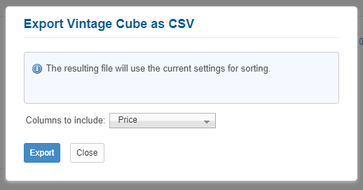
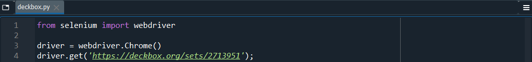
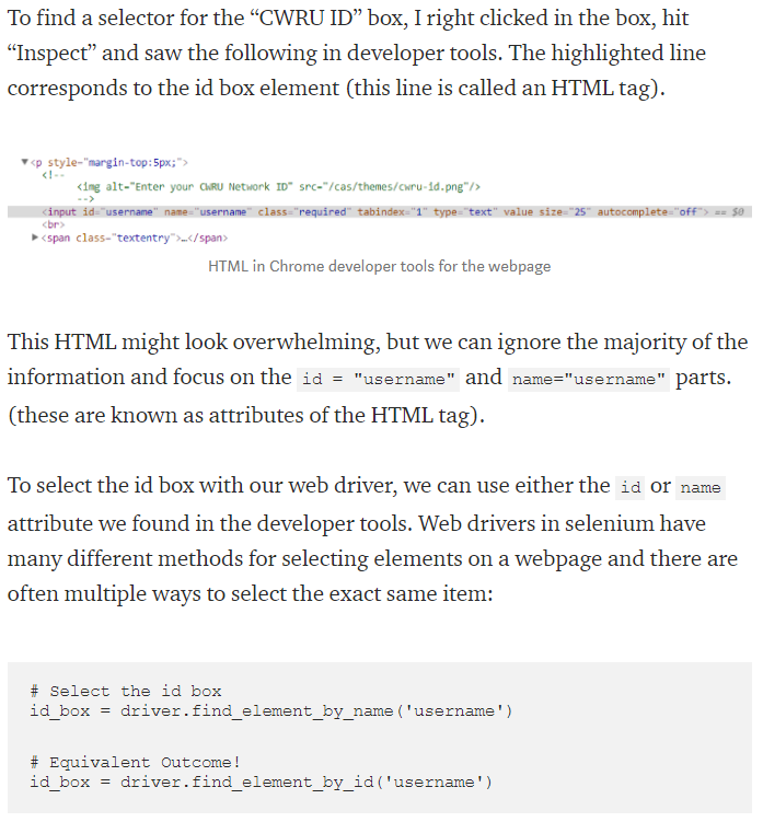
I have my magic the gathering collection on deckbox.org, which has an option allowing for the collection of cards and prices to be downloaded as a csv file.

Hovering over the Export button in the top right shows a dropdown option “Export to CSV”, which creates a pop-up. The pop-up has another dropdown, where the price can be selected to be included in the downloaded csv.

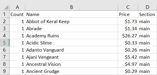
This generates a csv file that looks like this:
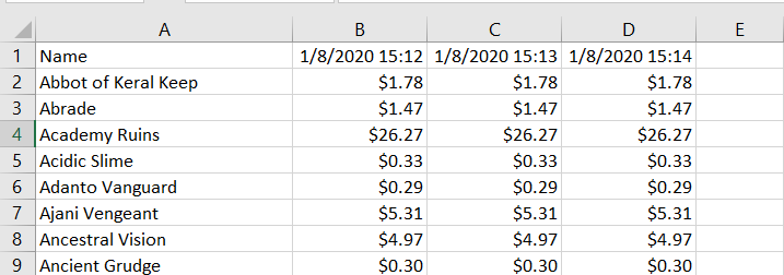
The goal is to write a script that queries the website daily for this csv file, and appends this set of prices to an existing csv file, along with a timestamp as a header:
I decided to use python, since python is really user friendly for projects like these. I happen to have very little experience with python, with maybe a few hundred lines of code written.
Since I know nothing about accessing the web with code, the first thing I do is google:

Clicking through a few links, I find this:

It seemed like there were a few options. Python has inbuilt functions for accessing and reading the text from websites, and several libraries exist that allow you to send HTML GET/POST requests. However, I don’t know much about HTML requests, especially not when it comes to their structure or formulation. I wasn’t sure if I would be able to easily input “Price” into the dropdown box through HTML POST requests.
Selenium seemed like a decent option, since it simulated the browser and let you click around and interact with the web objects, so that was what I decided to use. I already had python 3 installed through Anaconda, with the Spyder integrated development environment (IDE), so the first step was to install Selenium.
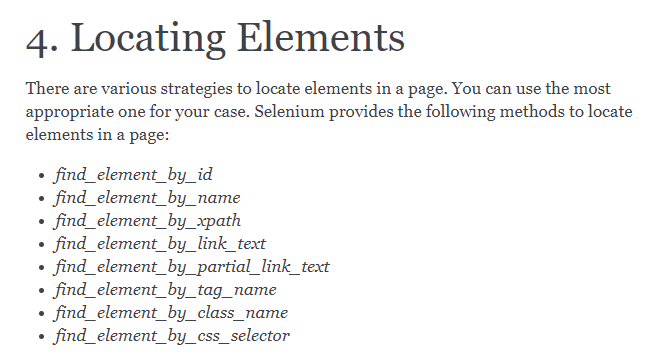
Setting Up Selenium
I start by googling:

And click on the installation link. This brings us to the documentations page for Selenium, which has a very helpful installation guide:
As instructed, I run pip install Selenium on my Anaconda prompt, and download the Chromium driver, since I use Chrome.
To test to see if everything works fine, I click on the getting started page on the Selenium documentation page, and run their sample code: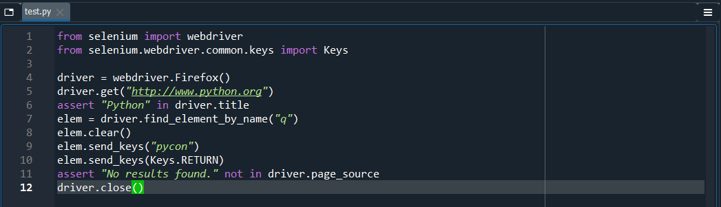
This gives me my first error:
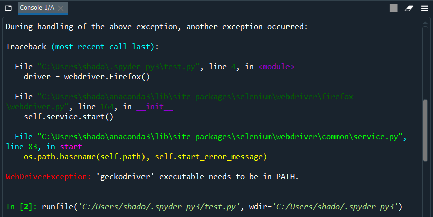
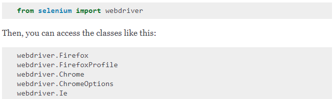
A quick google reveals that geckodriver is the Firefox driver. Taking a look back at the default code, we see that it calls webdriver.Firefox() instead of the Chrome equivalent.
![]()
A quick check back on the documentation shows that the correct function call for Chrome is webdriver.Chrome()
Editing my code and rerunning it gives a new error:
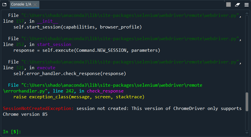
Googling this new error brings us to the following stack overflow thread:
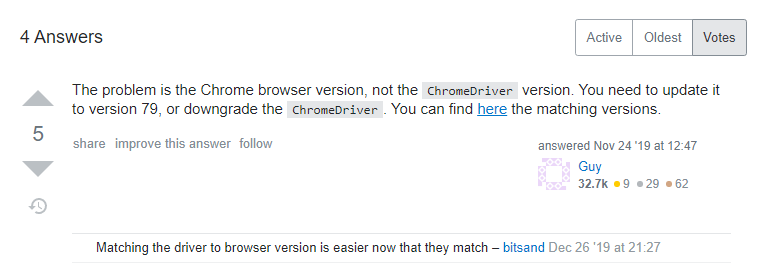
Checking the downloaded versions, I see that I have Chrome version 84 installed, but Chromium version 85 installed. Reinstalling Chromium version 84, and rerunning our program gives us our first taste of success:
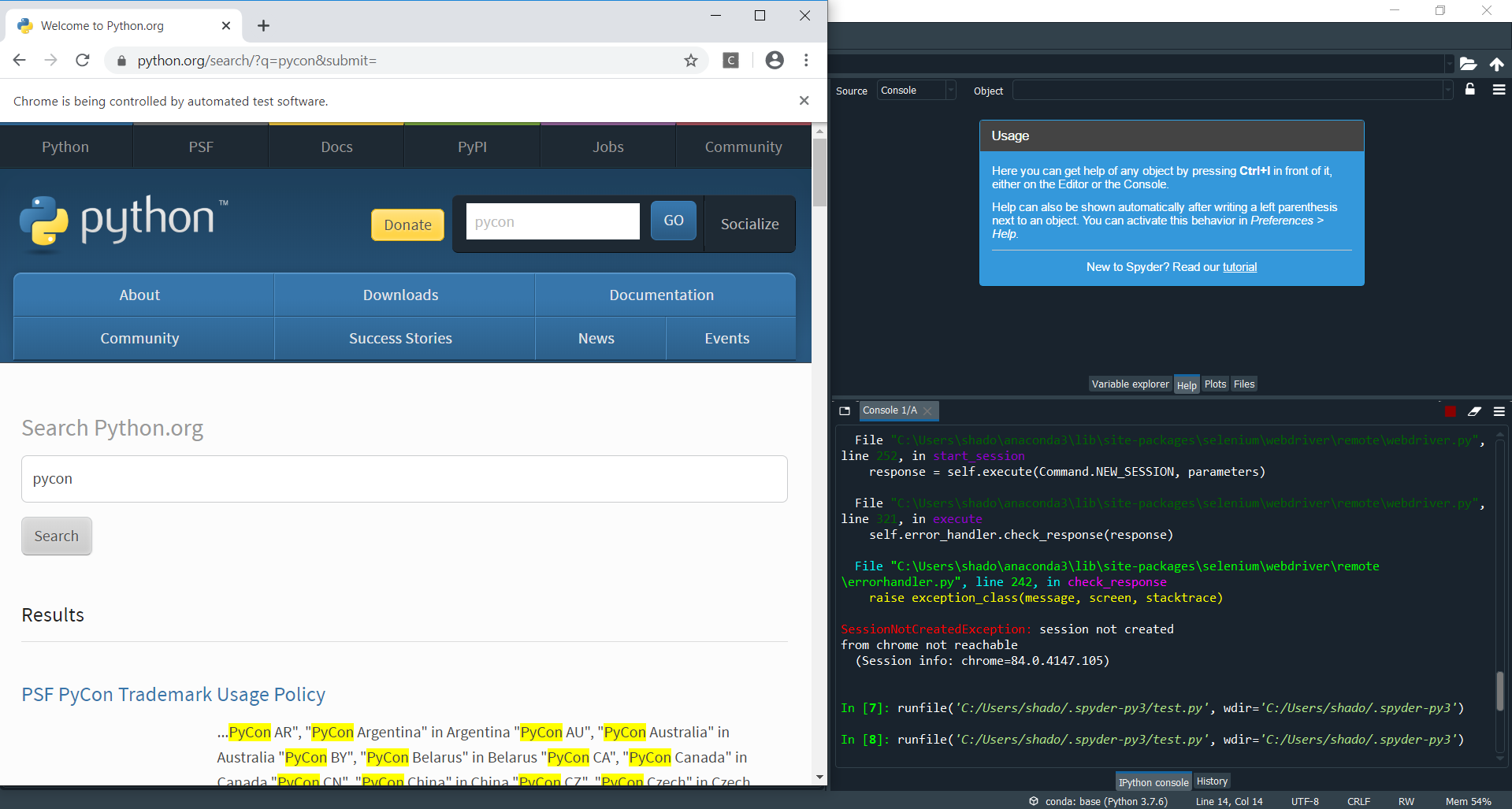
The python.org page loads! Now we know that our installation is working.
Downloading the Data
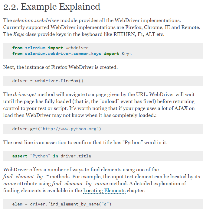
Now that we have Selenium installed and working, we need to figure out how to use it to access the site. I would usually google “Selenium tutorial” at this point, and look for an easy to understand guide with some code, but in this case, Selenium has a great detailed guide in their documentation site, so I’ll be using that instead. Although sometimes technical and hard to parse, these documentation sites are usually the best place to get detailed information about what the available functions are, and the syntax for these functions.
We take a look at the example provided by Selenium:
And their explanation of the example available here:
I also googled “selenium python web interaction”, and found this, a very useful walkthrough of Selenium, and how to use it. He included some code:
And a brief description of how Selenium worked:
Both these resources tell us the same thing, that the code to begin with is:
It also tells us how Selenium works. We have to use the functions Selenium provides to select an object, to then be able to click on it. Let’s take a look at how the guy does it:
Let’s try the same thing! Let’s inspect the element and see what tags we get:

Unfortunately, it doesn’t seem like this HTML has an id tag. How else can we select this element? Going back to the documentation, we see:
Since id and name don’t work, lets try searching for it by xpath. A quick google of “finding xpath in chrome” gives this stackoverflow thread:
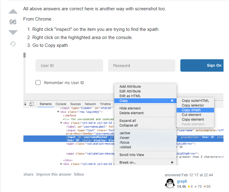
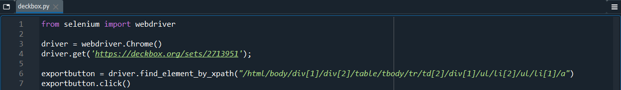
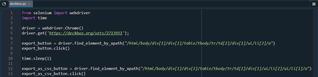
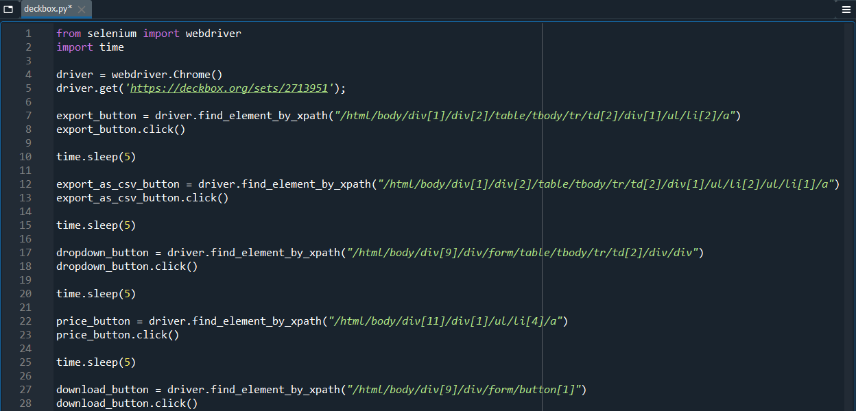
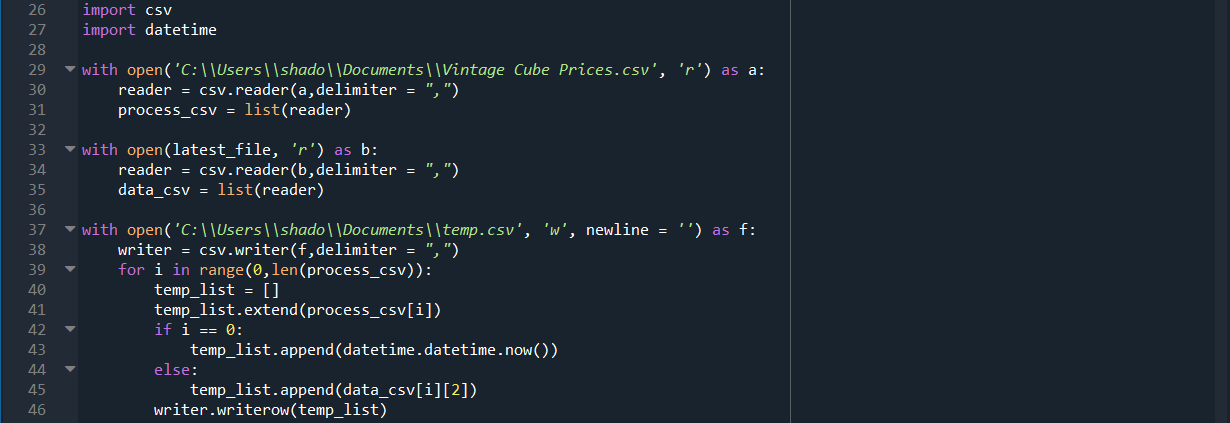
Repeating the same steps gives us the xpath: “/html/body/div[1]/div[2]/table/tbody/tr/td[2]/div[1]/ul/li[2]/ul/li[1]/a”
We want to click on this button to get our popup, so lets look for the click command in Selenium. A quick check on both our Selenium documentation and our walkthrough shows us that the command is just .click():

Adding this to our code gives:
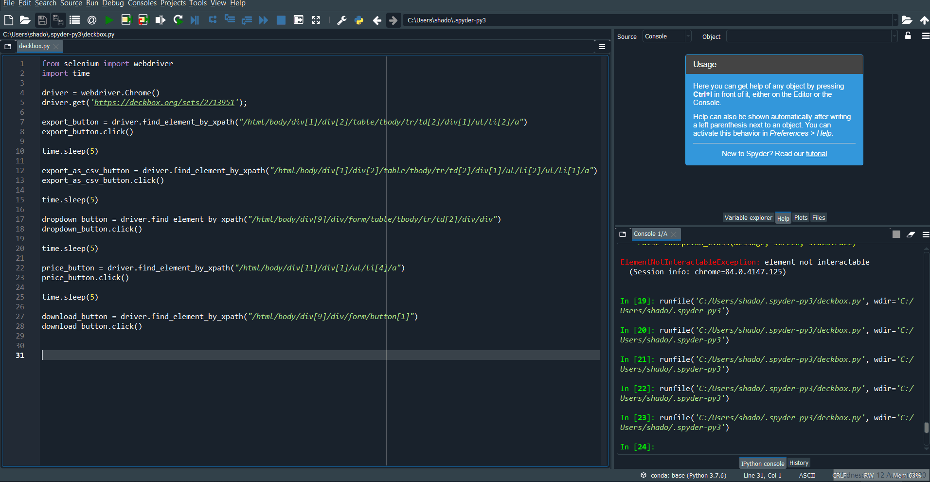
But this gives us another error message:
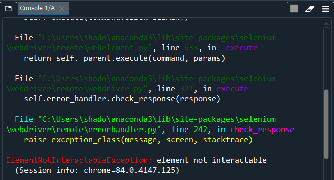
A quick google of “selenium element not interactable” gives us several stackoverflow threads about this error.
So here we learn something about how Selenium works. Selenium simulates a browser, and can only access elements that can be seen. To access the “Export as CSV” button, we first had to click on the “Export” button. Since we had not yet clicked on the “Export” button, the “Export as CSV” button was not visible, so we could not interact with it, giving us the error.

Fixing this problem is pretty straightforward, we find the xpath for the “Export” button, make sure we click on it first, and only after do we attempt to click on the “Export as CSV” button. Other threads also suggest adding a slight wait time so that the button has time to appear. Adding everything, we get:
Running it yields success! The popup appears.
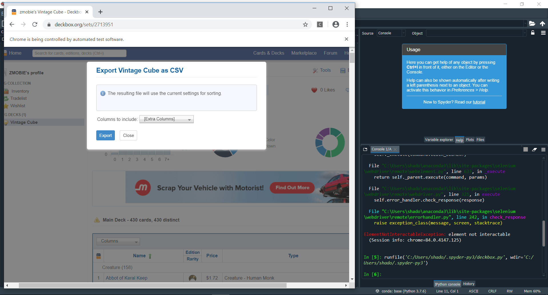
The next step is slightly different. Instead of a button, we now have to interact with the dropdown, to add “Price” as one of the Columns to include in our requested csv. It turns out that repeating the previous steps works. We can find the xpath for the dropdown box, the “Price” entry, and then the “Export” button, and click on each of them in turn.
Running it, we see that it downloads the desired file into our downloads folder.
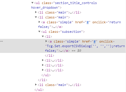
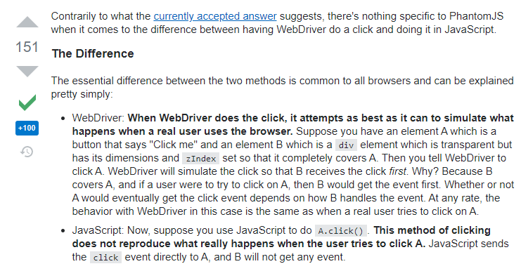
That is one way to obtain the downloaded file. What actually happened when I originally coded it was something slightly different. When I first ran into the “element not interactable” error, I mistakenly believed that the object could not be clicked. If we take a closer look at the html for the first “Export to CSV” button that creates the popup after clicked, we see the following bit of code:
![]()
It looked like it was running some kind of code with the “onclick = ” part, so I googled “onclick = “. This brought me to this site, which explained that it was running javascript.

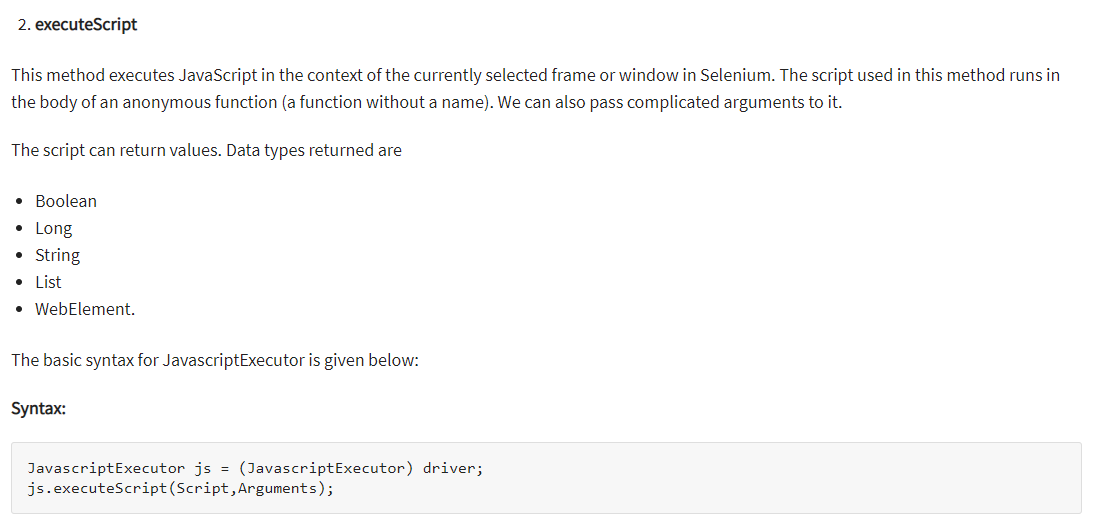
I next googled “selenium run javascript”, which brought me to here. Here, the syntax for executing javascript with selenium was available:
A quick google of “Tcg.Set.CSVDialog” gave nothing, which made it seem like this was a custom javascript function of the website. It didn’t seem likely that I would be able to find documentation on the exact usage, so I guessed a bit. I first tried executing the first line of javascript, to see what would happen.
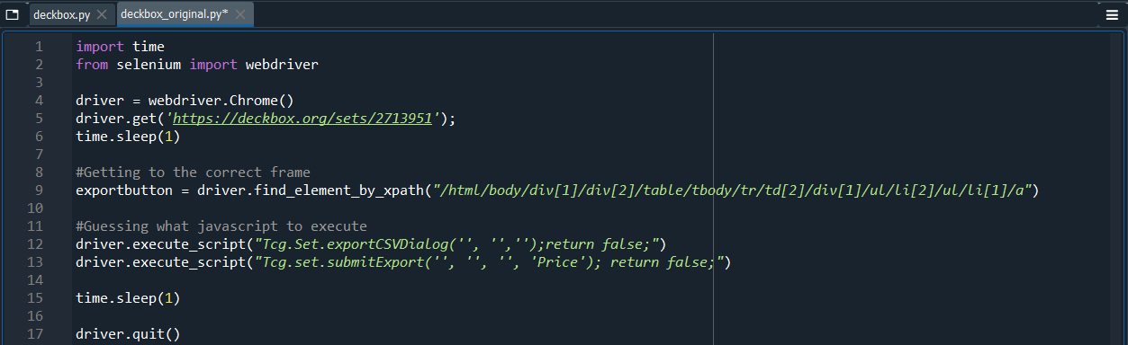
The first line of javascript was successful, and opened up the popup. To obtain the second line, I went back to looking at the html for the second Export button.

Again, I had to do a bit of guesswork. I wasn’t sure how I would get the “Price” Column included, but it seemed like the fourth entry of the submitExport function was the columns that had to be included in the downloaded file. I guessed that placing ‘Value’ there would work, tried it, and was greatly relieved when it did produce the desired csv file.
The coding process is oftentimes wrought with setbacks, and it is frequently not obvious how to continue with the project. A bit of luck with guessing around, or more in depth googling both help when stuck.
Updating our csv
After downloading the day’s new data, we still have to use python to append it to our old data.
First, we have to find the downloaded csv file. Selenium puts it in our downloads folder, but deckbox has it so that the file name has today’s date too. Annoying. A quick google of “most recent file python” brings us to this thread:
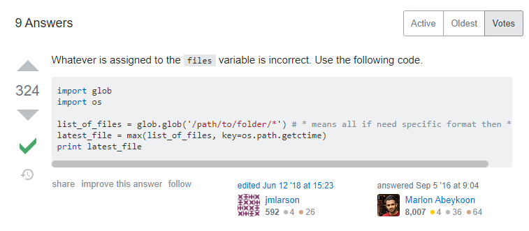
After changing the folder address to our downloads folder, we get an error:
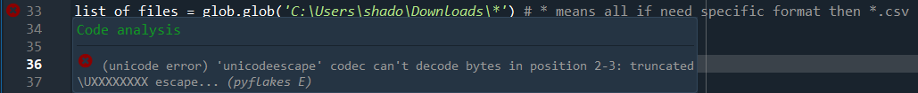
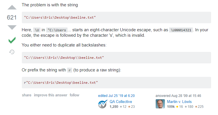
Googling “unicode escape python error” brings us to this thread, which explains that \U is a special escape sequence in python. Huh, TIL.
Duplicating the backslashes, and running the test code, we see the latest file name as output:
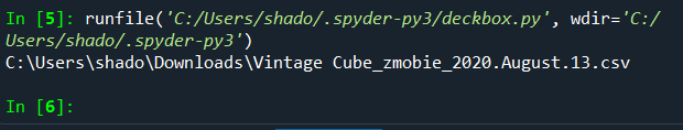
That’s great! This also tells us that the previous lines of code give us the full file address as output. We now have to append the Price column on this file onto our old file.
Finding resources on how to edit csvs is much easier, given how it is a much more prevalent problem. A quick look at google results of “append column csv python” brings us to this thread:
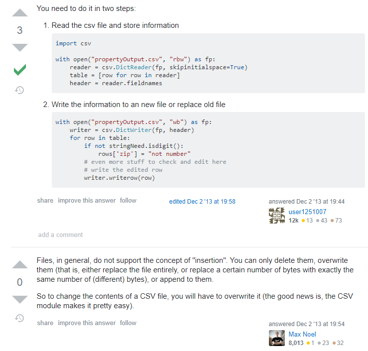
explaining how reading csvs work in python. Editing current files is not supported, and we have to rewrite into a new file. Further googling yields another with code similar to what we want:
Placing our file names in, and removing the superfluous length check (Turns out our downloaded csv from deckbox has an extra 4 blank lines) gives us the following code:
Running this code, we get the following error:
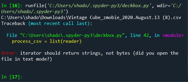
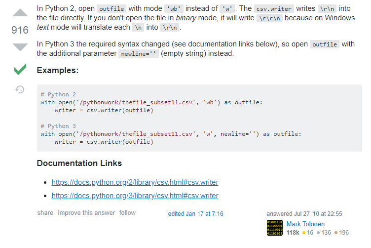
Googling “iterator should return strings, not bytes error python”, brings us to this solution:
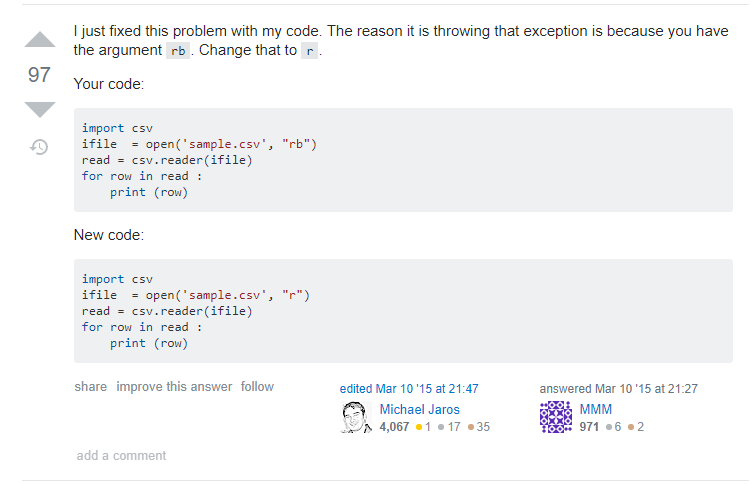
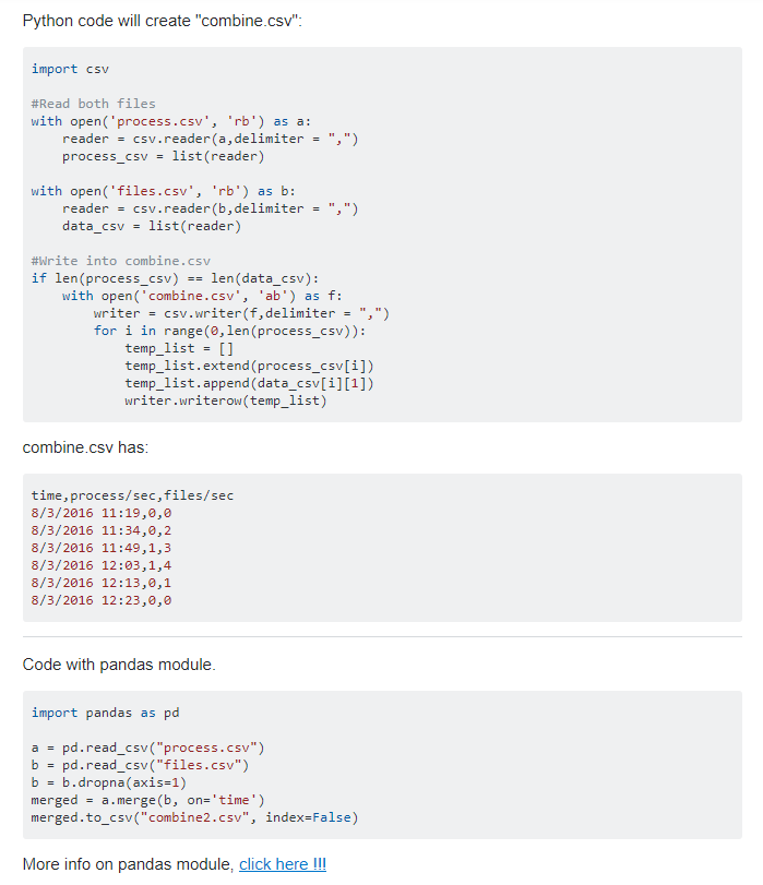
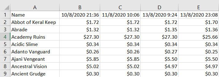
A quick change of all the “rb”s and “ab”s to “r”s and “a”s gives us a program that runs without errors. Let’s see what our output file looks like!
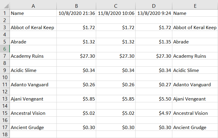
Not quite right. We copied the wrong column over, we didn’t change the header row to be the current time, and there are these blank rows. Let’s fix these problems one at a time.
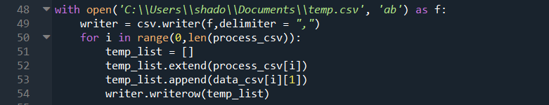
Let’s try and understand what the code is doing. At a glance, it looks like the code is iterating through each row, and creating each row by first creating an empty list “[]”, adding the original entries of “process_csv[i]”, then the “1” indexed column of “data_csv[i]”. Given that python uses 0 indexing, this corresponds to column B, explaining why the names are copied over. We should change this “1” to a “2” for column C, the price column.
For the first row, since we do not want “Price” to be copied over, we instead append the current time “datetime.datetime.now()” when i is 0.
Googling “csv blank rows python” brings us to this thread:
Oh huh, there is some unusual interaction with the way Windows reads newline characters. Our problem is easily fixed adding the newline = ‘ ‘ parameter. Running our new code:
Gives us our desired result, yay!
Our script works! For the final step, we want our script to run on startup, so lets google how to do that with “run python script on startup”. This brings us to this thread:

Placing the .bat file in the folder completes our project. A quick restart of our computer verifies that the process works.
This entire post might have been too excessively detailed, but I hope it shed some light on the coding learning process. For someone inexperienced with the nuances of the language, googling things and reading things on stackoverflow is a very normal part of the process. Sometimes, when you get stuck, trying a different approach, or doing a bit of guessing goes a long way.
 and
and  , if there is a zero knowledge proof that convinces the verifier if the two graphs are isomorphic. A description of this problem, as well as a solution to it is available in the link provided above. Reading it would provide some background for the strategies employed that follow.
 has the same distribution as sending two permuted versions of
  , can we construct a zero knowledge proof to demonstrate to the verifier that one of
  or
or  ? In particular, to provide some intuition as to the problem here, we are trying to construct a zero knowledge proof that does not reveal to the verifier which of the two graphs is the one isomorphic to
  . The verifier then sends back an integer, pointing to one of these two graphs, and the prover responds by providing the permutation from
  .
. that it itself constructed. This means that for the simulator to simulate the prover providing the permutation from
  in the case where the prover picks
  , and the simulator sends over
  , in the case where the prover picks
  . The simulator has to simulate both cases happening with probability half, for the correct distribution. However, in the event that one of the two graphs is not isomorphic to
  and
and  do not have the same distribution.
 in a random order. The verifier then randomly points to one of the three graphs, and asks the prover to show that this graph is isomorphic to
  if one of the graphs is isomorphic to
  if neither of the two are.


 is some random permutation of
  , that
  and
and  are indeed isomorphic to
 . The distribution of the above simulated graphs looks precisely like some combination where neither of the two

 blue points and

 time with the Hungarian algorithm.
 lines between any two points), we can perform a line sweep so that the number of points on either side of this line is exactly

 to
to  , so that at some time in between, it must hit 0. There are some minor details, such as if
  and
and  so that both sets have even number of points.
 with the desired angle, and finding the distances of each of the points to this line
  time, then using quick select to find the half of the points that belong on one side. This gives us
  time required for the divide and conquer step, and an overall time required of
  .
. . We want to look at the possible edge colorings of this graph. Suppose we know by Vizing’s theorem that an edge coloring with
  colors exists. Is there an edge coloring with the number of edges of each color being precisely either
  or
or  ?
? and
and  respectively. If we have that
  , then we know that if we consider the subgraph generated by
  . Where
  is the set of edges of color
  . Since the sum of the
  is constant, this is minimised when the
  time. We also see this in AVL trees, where maintaining the property that each node has children with heights differing by at most 1 guarantees a Fibonacci lower bound in size and hence a logarithmic bound in height.
 and
and  , with
  , we can consider a few cases for where our sampled
  , then no matter which card we picked, we would switch, and the chance of success is 50%. Likewise, if
  , then we would always keep the card we picked, so the chance of success is still 50%.
 we picked happened to be between the two values
  .
. pre-processing to store all distances for
  queries, or do
  pointers towards the root in the least common ancestor algorithm along with the distances for
  time. We also have to ensure that is it easy to find which segments we have to query. This is however relatively simple, since the path from a vertex to its least common ancestor with any other vertex passes through only from positions to ends of chains (going upwards), so determining which ranges to query is in fact easy.
![LPS[i] = k](https://s0.wp.com/latex.php?latex=LPS%5Bi%5D+%3D+k&bg=ffffff&fg=141412&s=0&c=20201002) if the longest palindrome centred around index
if the longest palindrome centred around index  (on each side).
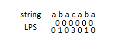
![LPS[x] > x - i](https://s0.wp.com/latex.php?latex=LPS%5Bx%5D+%3E+x+-+i+&bg=ffffff&fg=141412&s=0&c=20201002) ), we can take reference from
), we can take reference from ![LPS[2x - i]](https://s0.wp.com/latex.php?latex=LPS%5B2x+-+i%5D&bg=ffffff&fg=141412&s=0&c=20201002) to figure out what
to figure out what ![LPS[i]](https://s0.wp.com/latex.php?latex=LPS%5Bi%5D&bg=ffffff&fg=141412&s=0&c=20201002) is. There are two cases:
is. There are two cases: fits inside the large palindrome at index
 ![LPS[2x - i] < LPS[x] - (x - i)](https://s0.wp.com/latex.php?latex=LPS%5B2x+-+i%5D+%3C+LPS%5Bx%5D+-+%28x+-+i%29&bg=ffffff&fg=141412&s=0&c=20201002) ), then we have that
), then we have that ![LPS[i] = LPS[2x - i]](https://s0.wp.com/latex.php?latex=LPS%5Bi%5D+%3D+LPS%5B2x+-+i%5D&bg=ffffff&fg=141412&s=0&c=20201002) .
.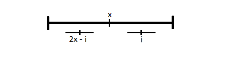 Case 2: If the palindrome at index
 ![LPS[i] >= LPS[2x - i]](https://s0.wp.com/latex.php?latex=LPS%5Bi%5D+%3E%3D+LPS%5B2x+-+i%5D&bg=ffffff&fg=141412&s=0&c=20201002) , and we will have to check what the actual value is.
, and we will have to check what the actual value is. 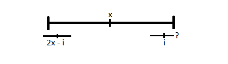 We now work on the LPS array in order using the above observation. We keep track of two things, the index
 ![x + LPS[x]](https://s0.wp.com/latex.php?latex=x+%2B+LPS%5Bx%5D&bg=ffffff&fg=141412&s=0&c=20201002) is maximal. There are
is maximal. There are  . How do we find all the vertices whose removal would cause the resulting graph to be disconnected?
 is only an articulation point if one of it’s sub-trees does not have a backward path going past
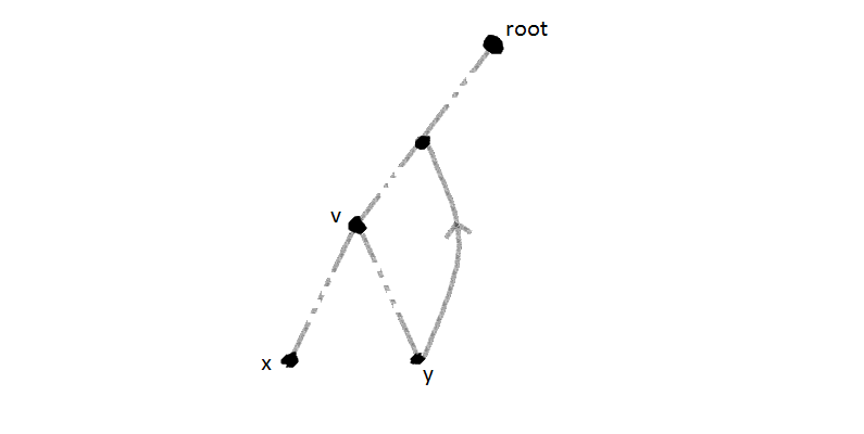
 , and had some path back up past
  time.
time. time, when we spend
  time, has
  fits in one machine word.
 , to count the number of unique indices we have visited already, we can solve this array construction problem in
  , so that when we are queried, we can figure out if the element at the position index is correct by linear searching through the second array.
 has been visited before, we store it’s position
  in a third array at position
  . If we partially order this set by inclusion, what can we say about the cardinality of these chains?
 . These sets form a chain in our poset, and the chain is of countable length.
 . Now, consider the sets
  . Each set
  is the set of natural numbers that maps to a rational number less than
  . Since this set is ordered by inclusion, and bijects to
  , we have an uncountable chain.
 to
to 